Deconvoluting spectra with pquad

This example shows how to deconvolute spectra using the model

The parity plot for the mixtures where concentrations are known is shown in figure 1 and the plot of concentration with time for the experimental spectra from reacting systems are shown in figure 2 and 3 for different starting concentrations

from __future__ import absolute_import, division, print_function
import os
import numpy as np
import matplotlib.pyplot as plt
from pquad import IR_Results
from pquad import get_defaults
from pquad.plotting_tools import set_figure_settings

Loading data

First, we’ll get the default data and load it into pquad. It automatically fits the model to the data in pure_data_path

frequency_range, pure_data_path, mixture_data_path, reaction_data_path = get_defaults()
deconv = IR_Results(4, frequency_range, pure_data_path)
mixture_data_path_file = os.path.join(mixture_data_path, os.listdir(mixture_data_path)[4])
deconv.set_mixture_data(mixture_data_path_file)
deconv_reaction = IR_Results(4, frequency_range, pure_data_path)
deconv_reaction.set_mixture_data(reaction_data_path, contains_concentrations=False)

Set figure settings

figure_folder='fit'
set_figure_settings('presentation')

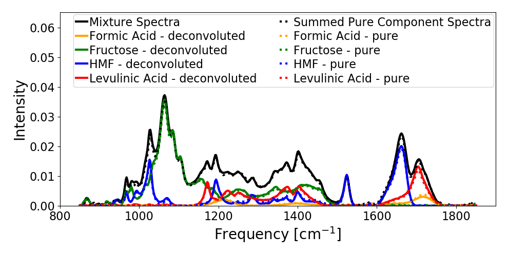
Plot deconvolution for mixture with known species-concentrations

Plot comparison of deconvoluted spectra and pure-spectra

deconv.plot_deconvoluted_spectra(figure_folder)

Out:

C:\Users\lansf\Box Sync\Synced_Files\Coding\Python\Github\pQUAD\pquad\pquad.py:802: UserWarning: Matplotlib is currently using agg, which is a non-GUI backend, so cannot show the figure.
  plt.show()

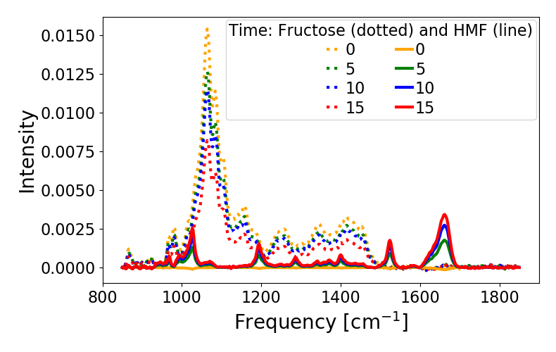
Plot deconvolution of Fructose and HMF during reaction

deconvouted_spectra = deconv_reaction.get_deconvoluted_spectra(deconv_reaction.MIXTURE_STANDARDIZED)
for i in range(deconv_reaction.NUM_TARGETS):
    if deconv_reaction.PURE_NAMES[i] == 'Fructose':
        fructose_index = i
    elif deconv_reaction.PURE_NAMES[i] == 'HMF':
        HMF_index = i
plt.figure(figsize=(7.9,5))
Colors = ['orange','g','b','r']
for count, spectra in enumerate(np.array(deconvouted_spectra[0])[:,fructose_index][0::5]):
    plt.plot(deconv_reaction.FREQUENCY_RANGE,spectra, color=Colors[count], linestyle=':')
for count, spectra in enumerate(np.array(deconvouted_spectra[0])[:,HMF_index][0::5]):
    plt.plot(deconv_reaction.FREQUENCY_RANGE,spectra,color=Colors[count], linestyle='-')
plt.legend([str(i) for i in np.arange(len(np.array(deconvouted_spectra[0])[:,fructose_index]))[0::5]] +\
            [str(i) for i in np.arange(len(np.array(deconvouted_spectra[0])[:,HMF_index]))[0::5]],title='Time: Fructose (dotted) and HMF (line)',ncol=2)
plt.xlabel('Frequency [cm$^{-1}$]')
plt.ylabel('Intensity')
plt.show()

Out:

C:\Users\lansf\Box Sync\Synced_Files\Coding\Python\Github\pQUAD\examples\deconvolution\plot_deconvolution.py:64: UserWarning: Matplotlib is currently using agg, which is a non-GUI backend, so cannot show the figure.
  plt.show()